Commodity trading markets are nuanced and complex, and trading organizations need to be able to interpret all available information.  This includes industry news and market prices, as well as information contained in price volatility and correlations between markets.  Volatility is not well understood by all market participants, in part because it is surrounded by mathematical mystery/intrigue.  Given recent market commotion, it is especially important for risk professionals to understand volatilities.  In this blog, we demystify the complexities around volatility by examining the different types of volatility, the mathematics behind volatility, and how traders and risk managers can protect themselves against downside and take advantage of new opportunities during volatile times (pun intended).

The Differences between Historical and Implied Volatilities

Most of us are aware of what price volatility refers to – it is part of our daily trading and investing lexicon.  Markets are said to be “volatile” when they go up and down dramatically, and most of us are barraged with headlines about stock and oil prices falling and (fingers crossed) rising again.  Most of these headlines refer to historical price action: what happened today or over the last month.  Financial engineers call this “historical volatility,” which is calculated from historical price movements.  We’ll discuss the math below.  Traders should understand the information contained in historical volatilities, even if they are not trading options.

However, historical volatilities are only part of the picture, and any trader who is only aware of historical volatility is like a driver who is only looking out the back window.  The options markets (whether for stocks, oil, or other commodities) also provide information about expected future price volatility.  This is called “implied volatility” because the volatility is implied by the observed prices of traded options. 

Historical and implied volatilities provide different information content.  Historical volatilities describe average or recent past price behavior, depending upon the sample period and/or choice of weighting method.  Implied volatilities represent supply and demand for options, and so are an indirect indication of the future volatility expected by market participants. 

We will provide a mathematical explanation of historical and implied volatilities below. 

Historical and Implied Volatilities Are Different But Related

Although historical and implied volatilities are usually different, they are also correlated, as illustrated by Tesla stock volatilities and prices during the last year (Images 1 and 2 from iVolatility.com).  There were periods when historical volatilities (HV) were higher than implied volatilities (IV), as well as the opposite – periods when implied volatilities were higher than historical.  In general, these represent periods when the market is less (or more) concerned about price changes, respectively.  Concern usually means the fear of a price drop.  This past January, for example, implied volatilities for Tesla were almost double historical volatilities.  This occurred during a period when share prices increased from $400 to $700/share, and implied volatility was signaling a fear of a sharp price drop (and expensive insurance against such a drop).  Next COVID-19 created market chaos, and both types of volatilities spiked.  But immediately after this price collapse, implied volatilities trended down from mid-March through April.  The fear that preceded the price drop was no longer present in the options market, making options (and insurance) cheaper.

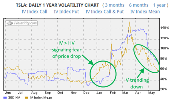Image 1: TSLA Daily 1 Year Volatility Chart, Source: iVolatility.com

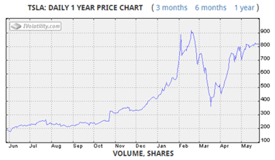Image 2: TSLA Daily 1 Year Price Chart, Source: iVolatility.com

A Volatility Metaphor: Would You Rather Believe a Historian or Economist?

In one of my earliest trading positions, I worked with a risk management consultant who taught me a valuable metaphor that applies to volatility.  To paraphrase him, understanding both historical and implied volatility information is like having a talented Ph.D. historian and Ph.D. economist on staff.  They may rarely agree about the meaning of available market information.  They may not even get along or like each other.  But there is value to be gained from their separate insights.

Let’s consider what our historian and economist are currently telling us about energy price volatility.  The following iVolatility.com  chart (Image 3) shows USO volatilities for the past year (USO is a leading oil ETF based on WTI futures for near-term delivery*).  Recent implied volatilities for USO are almost 50% lower than historical volatilities.  Implied volatilities are at their lowest levels since the March price collapse, and trending toward normal levels (below 50%).  The crude options market is projecting that crude price volatility will decrease from recent abnormal heights.  The trader and risk manager must decide – which is more indicative in our current environment, the 60% implied volatility or 120% historical volatility?  Should your risk system use one or the other or both?

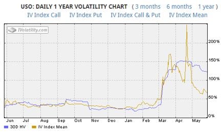Image 3: USO Daily 1 Year Volatility Chart, Source: iVolatility.com

*The USO ETF intends to approximate the return associated with the spot crude price, analogous to what a gold investor would achieve by purchasing gold bars or ingots.  USO attempts this by rolling positions in nearby futures contracts, which are not exactly the same as spot exposure.  In any event, its investors are displeased with its 75% loss during March and April, prompting both the SEC and CFTC to open probes into whether USO properly disclosed its risks.  However, commodity futures are not investment assets.  This reminds me of the old joke about “investing” in commodities – that the only difference between investing in commodities futures and investing in managed commodity funds is how fast you lose all of your money.

Note, when you compare historical and implied volatilities in this manner, that historical volatility naturally lags implied volatility because of the way it is calculated.  An event will continue to impact historical volatility as long as it remains in the sample period (30 days in the above example).  Techniques are available to reduce this lag effect (e.g. shorter sample periods, date shifts, or exponential weighting).

In contrast, recent implied volatilities for US natural gas futures have been significantly higher than historical volatilities, indicating that the options market is expecting price volatility to pick up significantly.  Image 4 is a plot of the 24-month forward term structure for both volatilities.  Implied volatilities also have more pronounced seasonal differences, particularly Jan-Feb 2021 and 2022.

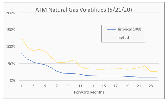Image 4: ATM Natural Gas Volatilities

Obviously, both trading and risk management teams would be very interested in the disparity (1.5-2x multiple) between these curves.  A trader should have a view as to which volatility is more likely to affect forward trades.  A risk manager may want to utilize both sets of data to evaluate market and/or credit risk.

Before discussing other information contained in volatilities, we will overview the math underlying volatility calculations. 

The Mathematics Behind Historical and Implied Volatilities

By standard convention, historical and implied volatilities for commodities are usually based on assumptions that are consistent with the Black 76 option model, adapted in 1976 by Fisher Black from the Black-Scholes equity option model.  The Bachelier model has also been in the spotlight recently and will be addressed later.

Historical volatilities are based on price changes for a sample period, usually the recent 20 or 30 business days, but longer sample periods may be used.  Short sample periods tend to represent current market conditions, but longer price periods (1 or more years) can be used to indicate average market behavior.  Percentage changes are calculated as the ratio P2/P1, where P1 is the price on the first day, and P2 on the next.  Next, the natural logarithm of this ratio is taken, ln(P2/P1).  These are referred to as “price relatives.”  This approach assumes log-normal price movements, which do not accommodate negative prices (more on that below).  Finally, the standard deviation of price relatives is calculated for the sample period (e.g. 20-30 days).  This standard deviation represents daily historical price volatility.  By standard convention (as in Images 1, 3, and 4), it is annualized by multiplying by the square root of 255 business days/year, since price is assumed to evolve as a function of the square root of time.  (useful rule of thumb: the square root of 255 is about 16, so you can easily convert daily to/from annual volatilities with a factor of 16.  A 4% daily volatility is about 64% annualized.)

Implied volatilities are calculated from traded option prices.  The most commonly used option pricing model for many commodity options is Black 76, for which value is a function of option type (call or put), price, price volatility, time to expiry, strike price, and interest rate.  For observed option prices, the price volatility can be implied if all other model inputs are known; hence it is called implied volatility.  Traditionally this is a recursive calculation.  For example:

• On May 28 WTI for July delivery settled at $31.94/bbl
• The call struck at $32 for July traded at $2.45/bbl. That option expires on June 17, in 21 days.
• Using the Black 76 model, a 70% volatility would price the option at $1.98/bbl, which is too low
• A 90% volatility would price the option at $2.58/bbl, which is too high
• Trial and error (or a recursive routine) would determine the implied volatility is about 86%, since this correctly prices the option at $2.45/bbl

But there’s a new sheriff in town.  Recent negative crude prices have shined a bright light on the limitations of the Black 76 model, which as mentioned above doesn’t accommodate negative prices.  The CME and ICE both recently replaced the Black 76 model for oil trading with the Bachelier model, a 120-year old technique which has experienced a recent resurgence.  It has been used since 2014 for interest rates, electricity, and natural gas options.  Several consequences of switching models are:

• The Bachelier model assesses higher values for out-of-the-money puts and lower values for out-of-the-money calls, since it permits negative prices and therefore a higher probability of price decreases than the Black 76 model with its underlying assumption of log-normal price movements.
• Its volatility is calculated from absolute, not relative moves as in Black 76. For example, the probability of a $10/bbl WTI price movement is the same whether the current WTI price is $30/bbl or $60/bbl.
• The Bachelier model characterizes volatilities in the same units as price, e.g. $10/bbl for WTI, instead of percentages.

These are relatively new developments, and integration of the Bachelier model in front and middle office processes is still underway at many firms.  Use of multiple models is likely here to stay, and these will create new challenges for trading organizations.

The Arbitrage Relationship Between Historical and Implied Volatilities

Now that we’ve covered the math behind historical and implied volatility calculations, we will consider their relationship further.  It is useful (although oversimplified) to think of implied volatility as a forecast of historical volatility.  This is because certain options are fairly priced if implied and historical volatility turn out to be equal.  If you buy an option, you are said to “pay” the implied volatility.  On the trade date, the implied volatility that you purchased represents a range of projected prices as illustrated in Image 5 (left).  Your payout will be a function of the actual (aka historical) price volatility, as pictured in Image 6 (right) for a large number of trials. 

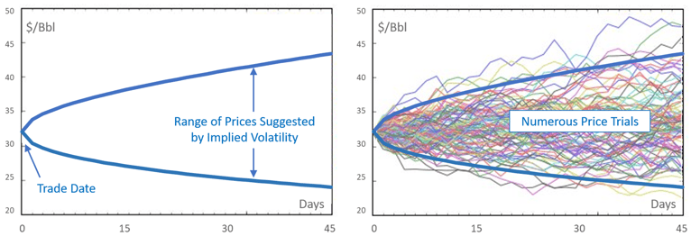Image 5 & 6: Arbitrage Relationship Between Historical and Implied Volatilities

If actual/historical price volatility turns out higher than the initial implied volatility, on average you will profit.  In Image 6, there is a greater chance that prices will stray outside of the expected range.  If actual/historical volatility is lower, on average you will lose.  In this case, you bought the volatility which was expected, but actual volatility turned out to be lower (well inside the expected range).  The opposite payouts apply if you sell options.  So implied and historical volatility are loosely related in this manner.

There are option trading strategies for which this arbitrage relationship is more direct.  One example is selling options that are delta-hedged with a linear position (e.g. equity or financial swaps).  As delta changes, the hedge must be adjusted.  When the option expires, the historical volatility which existed during the strategy had a strong impact on how often the hedge had to be adjusted.  If historical volatility was less than the original implied volatility which was sold, then the trade would tend to be profitable.  Conversely, historical volatility which was significantly higher than implied volatility would usually make such a strategy unprofitable.  The economics of this strategy are a strong function of this relationship between implied and historical volatilities, although there are also other financial impacts (i.e. fees and gamma effects).  Similar trading strategies can be used to arbitrage the difference between historical and implied volatility.  In fact, this arbitrage is implicit to many volatility-based trading strategies (i.e. any strategy with vega, which is what option traders call exposure to volatility changes).

Contango and Backwardated Volatility

The natural gas volatility curve in Image 4 demonstrated a negative (backwardated) slope.  This is a phenomenon that is common for commodities and is a consequence of the option model (Black 76) which underlies the volatility assumptions.  In this model, prices are assumed to evolve as a function of the square root of time, but this overstates commodity market behavior.  The market indicates (through historical and implied volatility levels) its belief about appropriate price distributions.  Image 7 compares 1-standard deviation price ranges for:

• Constant volatility – price bands are calculated based on the 125% prompt implied volatility on Image 4 applied to all delivery periods (or option tenors) multiplied by the square root of time
• Forward volatilities – price bands are calculated using the same approach, except that (lower) forward volatilities for each delivery period are substituted for prompt volatility. These are the forward implied volatilities from Image 4.

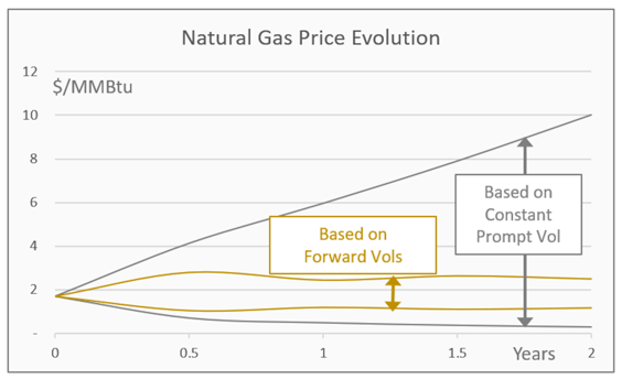Image 7: Natural Gas Price Evolution 

Image 7 demonstrates that the market is projecting a much tighter range of likely future prices, than the constant volatility price bands would predict.  For example, the 125% prompt implied volatility suggests a $0.50-$6.00/MMBtu price range after only 1 year.  The implied volatilities for the 12-month future, only 36%, imply a much tighter price range of $1.20-2.45/MMBtu.  In effect, the markets are communicating expected forward price distributions through these implied volatilities.

Most widely traded commodities options relate to individual forward delivery periods, and they are valued using volatilities and other data specific to that period.  More complex path-dependent options, e.g. barrier options, require pricing models that evolve spot prices to generate reasonable future price distributions, such as illustrated in Image 7.  This is a difficult problem.  Such models often use mean reversion mechanisms or multiple volatility factors to manage the phenomena illustrated in this chart.

Some markets behave differently.  For example, equities often have a constant volatility term structure, implying that prices could evolve more rapidly, similar to the constant volatility range in Image 7.  Equities are thought to lack a price ceiling, and are also more likely than commodities to lose all value (notwithstanding recent WTI prices).  Sometimes equity volatilities have a contango volatility structure, particularly when impactful news is expected soon (e.g. earnings announcements or FDC drug trial results).

Volatility Smiles and Surfaces

So far we have considered one dimension of volatility term structure, delivery period, but another dimension is “moneyness.”  Moneyness is usually defined as the ratio of strike to underlying price, the “log strike” (logarithm of strike/price), or option delta.  Image 4 displayed only at-the-money volatilities.  For a single delivery period, if we plot volatility as a function of the other dimension, moneyness or log strike, we often observe the “smile” shown in the following chart.  Image 8 is an old chart (2013), but a favorite of mine since it compares equity and WTI volatilities.

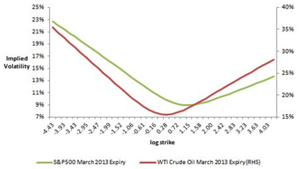Image 8: Equity vs. WTI Volatilities, Source: SeekingAlpha.com 

This chart begs several questions – First, what does the volatility smile tell us?  As before, it is useful to consider what constant volatilities would suggest.  The Black 76 model assumes a log-normal distribution of prices, and horizontal (constant) lines on the above chart would suggest that price changes are log-normal.  Higher implied volatilities for options that are in- or out-of-the-money imply that they are more valuable because these price outcomes are more likely.  This means that options traders are associating a higher probability of tail events than suggested by a log-normal distribution; financial engineers call this kurtosis or heavy tails.

Second, why is the smile different for equities and commodities?  The equities smile is sometimes called a “smirk” since it is biased toward lower strikes.  The equity options market is primarily driven by supply and demand for insurance against price drops; thus lower strikes are more valuable than higher strikes.  The commodities markets are more balanced between producers and consumers, making low and high strikes somewhat equally valued.  Occasionally, commodity markets will also experience short or long term effects that create smirks, e.g. hurricanes in the Gulf of Mexico or unscheduled refinery outages.

Now that we’ve discussed smiles, we should note that the “new” Bachelier model doesn’t smile much.  A recent article in Risk.net, Bachelier – a strange new world for oil options, presented the following comparison of Black 76 and Bachelier, immediately before the negative WTI price events in late April.  Note that the Bachelier model implied volatilities are more constant functions of strikes, indicating they better model the “tails” of the oil price distribution.

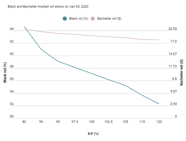
Image 9: Black 76 and Bachelier Comparison, Source: Risk.net

The combined effect of delivery period (or tenor) and moneyness on volatilities is referred to as the volatility “surface.”  An example of a 3-dimensional volatility surface is illustrated in Image 10.

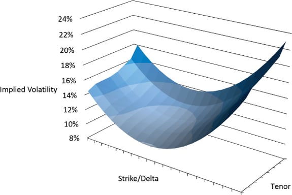Image 10: Three-Dimensional Volatility Surface Example, Source: O'Reilly

Although this section has focused on implied volatility surfaces, significant differences exist between historical and implied volatility surfaces.  These differences represent important trading and risk management signals.

Volatility Can Be Counter-Intuitive

We should keep in mind that volatility doesn’t always behave as expected.  Outside of plain-vanilla options and very controlled situations, I have found intuition is difficult to develop.  Several examples of unexpected outcomes include:

• Spread options whose calculated value decreased on days that the volatility of both underlying commodities increased (due to correlation changes)
• Owned or leased storage options that had negative vega (usually impossible for long options)
• Traditional option models that don’t function with low or negative prices.

The sometimes controversial Nicholas Taleb, author of Black Swan, has written interesting material on the unexpected characteristics of volatility and uncertainty.  Depending on your level of interest, several thought-provoking reads are:

• His 2007 paper with Daniel Goldstein, We Don't Quite Know What We Are Talking About When We Talk About Volatility
• His 2001 book, Fooled by Randomness, The Hidden Role of Chance in Life and in the Markets

Risk Managers and Middle Office: Update Your Risk Management Frameworks

The types of information that we’ve reviewed in historical and implied volatilities have obvious implications for traders, but what about risk managers and the middle office?  Veritas believes it is equally important that your risk management framework incorporates this information.  Several examples of practical applications include:

• Risk analysis (market and credit) can make use of two or more datasets that encompass reasonable ranges in volatilities.
• Alternatively, 1 or more historically derived input datasets can be used, as well as a dataset consisting of implied volatilities and correlations. Typically, the latter requires some subjective assumptions (since a full set of implied volatilities and correlations cannot be observed for all markets), but results can be informative in combination with other more objective analyses.
• Estimated error can be calculated for market and/or credit risk based on a range of input data (such as volatilities) and/or other time-varying input. Error estimates are an explicit recognition that risk varies significantly and unpredictably over time.
• Scenarios can be developed based on dramatic changes in markets.

Another advantage of multiple risk models and error estimates is they dissuade executive stakeholders from thinking of risk estimates as a single precise number, e.g. $15.137 million, and instead as a range of possible outcomes, e.g. $12-20 million, which depend on specific market assumptions. 

Summary

This blog attempts to compare historical and implied volatility, as well as discuss other volatility characteristics that are important to commodity traders and risk managers.  Veritas believes that it is important to understand the differences between historical and implied volatility, as well as when and why they converge or diverge.  This leads to better trading strategies and more robust risk management frameworks. 

After all, how many of us included minus $37/barrel in our WTI VaR or scenario estimates before April?

At Veritas Total Solutions, our team of experts is versed in trading & risk advisory capabilities. We offer advisory services in commercial strategy, organizational structure and capabilities, and technology solutions. If you are interested in learning more about our capabilities, contact us to learn more or subscribe to our blog to stay connected!