Value at Risk (VaR) has been in the spotlight recently, following several dramatic market drops. The VaR methodology is regularly criticized during periods when market volatility increases sharply. It’s easy to find quotes by portfolio managers and risk professionals that claim their risk systems are misfunctioning and place the blame at the foot of mathematical models. The journalism is sometimes overly simplified, but experienced risk professionals are not surprised by the difference between modeled and actual results.

However, we believe that it’s important to debate VaR’s practice and usefulness, so we’ll offer our perspective. Several important points are underscored by recent events:

1. VaR models based purely on historical market statistics offer little predictive capability,
2. VaR models based on implied volatility provide additional information in certain market conditions, and
3. All VaR models are imperfect and will under or overestimate risk for prolonged periods.

In our view, this is not a question of models being right or wrong, but it’s very important to understand their tendencies in different market conditions. Let’s take a look at recent activity in several markets to explore these points further.

This blog presumes knowledge of historical and implied volatility. For additional background, you can refer to our blog, What are Historical and Implied Price Volatilities Telling Us?.

Example #1: Recent S&P 500 Market Risk

We’ll use the U.S. equity market for our first example. The following charts show recent prices for SPY (a popular ETF mirroring the S&P 500), as well as SPY historical and implied volatility (from iVolatility.com).

Early in the COVID-19 pandemic, the S&P 500 fell 34% in just over one month (Chart 1, Period A), then rapidly recovered 2/3 of its loss (Period B). Continued market strength pushed the market above pre-pandemic levels, until a recent 8% pullback (Period C).

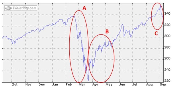Chart 1: SPY ETF Price

Chart 2 depicts volatility (historical and implied) during the same period. Although neither volatility predicted the large drop in February and March, you can see during Periods A and B that very different information was communicated by historical and implied volatility. As the market fell (Chart 2, Period A), implied volatility predicted significantly more risk than the trailing historical calculation. When the market began to recover (Period B), fear left the options market and implied volatility was at times half the historical level. Recently (Period C), implied volatility signaled concerns of another pullback. Although volatility levels were much lower since August than during March and April, it is still notable that implied volatilities during August were 1.5-2.0 times higher than historical volatilities.

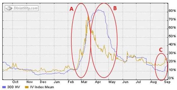
Chart 2: SPY ETF Historical and Implied Volatility

Most VaR models are based on a recent historical sample period, e.g. daily price returns over the past 3 months. When a string of sudden bearish or bullish moves occur in the market, these models trail actual impacts. As illustrated above, an additional VaR calculation based on implied volatilities may provide a significantly different perspective which a risk manager should consider.

Here we are comparing implied volatility with a 30-day historical volatility, which is essentially a 1.5 month unweighted moving average.  It is common practice to use exponentially weighted moving averages (EWMA) to bias the risk statistics toward more recent market action.  This has several Pros and Cons:

• Pro: Market changes are more rapidly incorporated in VaR or other analyses, approaching (but not equaling) the information content of implied volatility.  This is particularly valuable as an additional scenario compared to longer historical sample periods.
• Pro: It reduces the impact of large market changes as they exit the historical sample period, since distant data receives lower weights.  This avoids the stair-step appearance of unweighted moving averages.
• Con: It decreases the information content of the historical data, e.g. effectively reducing a 60-day sampling period to the 15-20 most recent days.  This can cause other mathematical challenges if positive definite correlations must be extracted from the data. 

Example #2: Back Test Reporting

In addition to the above qualitative observations, we can use a Back Test report to determine how many times actual market returns would have breached VaR limits calculated with historical versus implied volatilities. We will continue to use SPY as the basis of the example as we did above. Chart 3 compares daily returns and risk during mid-February through the end of April 2020 for a long position in SPY.

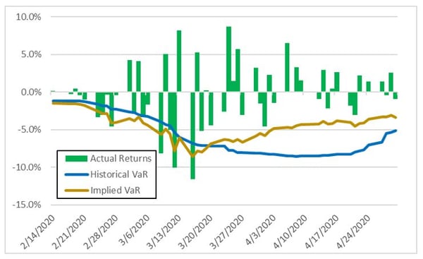
Chart 3: SPY Back Test Report (Daily Returns vs. 95% VaR)

It can be argued that VaR calculated from implied volatilities was more realistic in both falling and recovering markets, although it’s interesting to compare both VaR methods to actual returns.

• Market can be riskier than predicted – From mid-February to mid-March when the market was dropping, VaR based on implied volatilities was exceeded fewer times than that based on historical volatility (6 vs. 9 breaches). Both models were breached more frequently than the single occurrence expected for a 95% confidence level. This means that the market was riskier than estimated by either calculation during this period, which should not surprise anyone. Sometimes this happens.
• Market can be less risky than predicted – In the following 1.5 months when the market was recovering, returns did not exceed either VaR method, although the “Implied VaR” was lower (based on absolute value) and closer to actual returns. Sometimes the market is less risky than the models predict.

There’s a common misperception that Back Test reports are only useful to validate models during system projects, such as the implementation of a new risk solution. We believe that they are also helpful in daily operations, to promote comparison and understanding of the differences between market action and risk estimates.  Back Test reports should be regularly monitored to track whether the number of limit breaches are reasonable, in order to determine if the VaR model accurately reflects the market and price distributions. In the examples noted above, neither the historical nor implied VaR models are “broken,” they are just providing different information. And sometimes you need to pay attention to what implied volatility is telling you.

Example #3: Recent WTI Market Risk

Next, we’ll look at recent 2020 price action for USO, an ETF based on nearby WTI futures. Charts 4 and 5 provide price and volatility charts since oil prices collapsed in March-April and partially recovered. We’ll compare historical and implied volatility for four different periods of time:

• February and early March (Charts 4 and 5, Period A) – during the runup to the worst price collapse, implied volatility was signaling concern about increased price uncertainty. VaR produced from implied volatility during this period would have been 20-40% higher than historical volatilities.
• Mid-March and April (Period B) – implied volatility (100-250%) was much more erratic than historical (120-150%). Implied volatility’s highest levels immediately preceded significant drops in WTI price.
• May and June (Period C) – WTI prices stabilized and slowly strengthened. During most of this period, implied volatility was significantly lower than the trailing historical volatility.
• August (Period D) – implied volatility increased again relative to historical volatility, in advance of the price drop in early September.
  

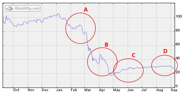
Chart 4: USO ETF Price

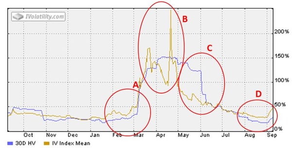
Chart 5: USO ETF Historical and Implied Volatility

“Avoid Explosions” by Considering Both Models

Healthy risk management organizations routinely debate the meaning of different models as described in these examples. True, with 20-20 hindsight it’s easy to pick periods like these, during which one methodology outperforms the other. However, no VaR models have perfect predictive capabilities. The question is, how do we make the best information available to manage our risks? Historical volatility (and VaR calculated from the same) is by definition a trailing indicator. In contrast, implied volatilities provide insight into the expectations of option traders, who are imperfect but at least attempt to predict future price action. Our main point is that these models provide different information. Your choice of whether to use one or both of these models or a more sophisticated predictive risk algorithm should be right-sized for the needs of your business.

It is non-trivial to implement VaR (or credit risk) models that are based on implied market statistics.  In many financial and commodity markets, implied volatilities and correlations are not continuously observed and it is difficult to obtain complete data sets.  It is often necessary to employ more complex processes to fill data or otherwise develop reasonable risk statistics.  These tend to require judgment and be more subjective, whereas risk managers prefer objective measures which cannot be manipulated.  There is not a perfect solution to this balancing act, and compromises may be required.  For this reason some organizations rely on historically based models as a “base case,” and use implied models as scenarios that provide additional information.

Standard VaR implementations are only reasonably accurate for +/- 1 standard deviation price movements, but they are attempting to describe risk beyond 1.6 or more standard deviations.  They also assume symmetrical probability of up/down market movements.  Both of these shortcomings can be addressed by scenarios, which should be used to augment the results of VaR in a comprehensive risk management process. Scenarios can include larger price changes (e.g. +/- $10-20/barrel) and directional shocks (e.g. +$5,000/MWH).

One of my undergraduate chemical engineering professors was fond of saying, “Your main job is to avoid explosions.” Similarly, one of the most important goals of risk management is to avoid surprises. The best way to manage the expectations of senior executive teams and other stakeholders is to promote a clear understanding of what risk models do and do not predict. Transparency and deep understanding are in everyone’s interests. Ideally, this will reduce the chance that your VaR model is ever blamed for poor financial results.

To read more about VaR, check out the other blogs in the VaR series: 

• Value at Risk (VaR): Overview and Benefits Case
• Successful Implementation of a VaR Solution 
• Refinery Risk Management and VaR Modeling 

At Veritas Total Solutions, our team of experts is versed in VaR and other trading & risk advisory capabilities. We offer advisory services in commercial strategy, organizational structure and capabilities, and technology solutions. If you are interested in learning more about our capabilities, contact us to learn more or subscribe to our blog to stay connected!